Plik:Jordan illustration.png
Przejdź do nawigacji
Przejdź do wyszukiwania
Rozmiar podglądu – 634 × 599 pikseli. Inne rozdzielczości: 254 × 240 pikseli | 508 × 480 pikseli | 812 × 768 pikseli | 1064 × 1006 pikseli.
Rozmiar pierwotny (1064 × 1006 pikseli, rozmiar pliku: 55 KB, typ MIME: image/png)
Opis
| Opis |
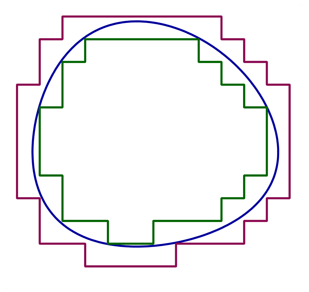
English: A set (represented in the picture by the region inside the blue curve) is Jordan measurable if and only if it can be well-approximated both from the inside and outside by simple sets (their boundaries are shown in dark green and dark pink respectively). |
| Data | |
| Źródło | Praca własna |
| Autor | Oleg Alexandrov |
| PNG rozwój |
Licencja
| Ja, właściciel praw autorskich do tej pracy, udostępniam ją jako własność publiczną. Dotyczy to całego świata. W niektórych krajach może nie być to prawnie możliwe, jeśli tak, to: Zapewniam każdemu prawo do użycia tej pracy w dowolnym celu, bez żadnych ograniczeń, chyba że te ograniczenia są wymagane przez prawo. |
Source code (MATLAB)
function main()

   % the function whose zero level set and inner and outer approximations will be drawn
   f = inline('60-real(z).^2-1.2*imag(z).^2-0.006*(real(z)-6).^4-0.01*(imag(z)-5).^4', 'z');

   M=10; i=sqrt(-1); lw=2.5;
   figure(1); clf; hold on; axis equal; axis off;

   if  1==0
      for p=-M:M
	 for q=-M:M
	    z=p+i*q;
	    if f(z)>0
	       plot(real(z), imag(z), 'r.')
	    else
	       plot(real(z), imag(z), 'b.')
	    end
	 end
      end
   end

% draw the zero level set of f
   h=0.1;
   XX = -M:h:M; YY = -M:h:M;
   [X, Y] = meshgrid (XX, YY); Z = f(X+i*Y);
   [C, H] = contour(X, Y, Z, [0, 0]);
   set(H, 'linewidth', lw, 'EdgeColor', [0;0;156]/256);

% plot the outer polygonal curve
   Start=5+6*i; Dir=-i; Sign=-1;
   plot_poly (Start, Dir, Sign, f, lw, [139;10;80]/256);

% plot the inner polygonal curve
   Sign=1; Start=4+5*i;
   plot_poly (Start, Dir, Sign, f, lw, [0;100;0]/256);

%  a dummy plot to avoid a matlab bug causing some lines to appear too thin
   plot(8.5, 7.5, '*', 'color', 0.99*[1, 1, 1]);
   plot(-4.5, -5, '*', 'color', 0.99*[1, 1, 1]);

   saveas(gcf, 'jordan_illustration.eps', 'psc2');

function plot_poly (Start, Dir, Sign, f, lw, color)

   Current_point = Start;
   Current_dir   = Dir;

   Ball_rad = 0.03;

   for k=1:100

      Next_dir=-Current_dir;

      % from the current point, search to the left, down, and right and see where to go next
      for l=1:3
	 Next_dir = Next_dir*(Sign*i);

	 if Sign*f(Current_point+Next_dir)>=0 & Sign*f(Current_point+(Sign*i)*Next_dir) < 0
	    break;
	 end
      end

      Next_point = Current_point+Next_dir;

      plot([real(Current_point), real(Next_point)], [imag(Current_point), imag(Next_point)], 'linewidth', lw, 'color', color);

      round_ball(Current_point, Ball_rad, color'); % just for beauty, to round off some rough corners

      Current_dir=Next_dir;
      Current_point = Next_point;

   end


function round_ball(z, r, color)
   x=real(z); y=imag(z);
   Theta = 0:0.1:2*pi;
   X = r*cos(Theta)+x;
   Y = r*sin(Theta)+y;
   Handle = fill(X, Y, color);
   set(Handle, 'EdgeColor', color);

|
Ta grafika (math) (lub wszystkie grafiki w tym artykule bądź kategorii) powinny zostać przetworzone na grafiki wektorowe jako plik SVG. O zaletach grafik wektorowych można przeczytać na stronie Commons:Media for cleanup. Jeśli wersja SVG tej grafiki jest już dostępna, załaduj ją. Po załadowaniu SVG zamień ten szablon na stronie tej grafiki na szablon {{vector version available|nazwa nowej grafiki.svg}}.
|
Historia pliku
Kliknij na datę/czas, aby zobaczyć, jak plik wyglądał w tym czasie.
| Data i czas | Miniatura | Wymiary | Użytkownik | Opis | |
|---|---|---|---|---|---|
| aktualny | 18:27, 4 lut 2007 | | 1064 × 1006 (55 KB) | wikimediacommons>Oleg Alexandrov | Made by myself with Matlab. {{PD}} |
Lokalne wykorzystanie pliku
Poniższa strona korzysta z tego pliku: